A Survey of Visual Noise Used in Graphics Programming and Design

In typical fashion, I decided to start a side project to assist in the development of another one of my side projects. This secondary side project was to create a generative noise plugin for the animated sprite editor & pixel art tool aseprite. The source code for the plugin can be found at noise.aseprite-extension.

I entered this project with surface-level knowledge about some of the more common noise functions used in graphics. I left with slightly more than surface-level knowledge and an awareness of many misconceptions about the subject that I had.

This post is meant to give an intuitive, hand-wavy sense for some noise functions with special focus on areas where I had misconceptions to hopefully speed up any reader's entrance to the field.

Contents

1. Perlin / Simplex / Gradient Noise
   1. Background
   2. Algorithm
   3. Examples
2. Voronoi Noise
   1. Background
   2. Algorithm
   3. Examples
3. Worley Noise
   1. Algorithm
   2. Examples

Perlin / Simplex / Gradient Noise

First, let's establish the difference between the three noises in the header.

1. Perlin. The "original" gradient / lattice noise developed by Ken Perlin. Creates smooth (continuous) noise generally in Euclidian space.
2. Simplex. An improved Perlin noise algorithm (also invented by Perlin) intended to have similar effects to the original, but with better performance and more even distribution over its range of $[0,1]$.
3. Gradient noise. AFAIK this is a term used to refer to a class of algorithms characterized by the use of gradients, as originally seen in Perlin noise. There are also many algorithms with the same effects as Perlin noise that make use of evenly-spaced gradients but take a different approach to calculation.

Lattice Noise. As far as I am aware, lattice noise is just meant to refer to any noise generation method that makes use of a lattice data structure in its generation. Often you will see that each corner of the lattice has a unique hash so that whatever value is associated with that cell can be recalculated on demand. Perlin noise uses a lattice structure by assigning gradients at each integer coordinate / corner of a lattice cell in a space.

Background

The main benefit of a function like Perlin noise is that it is smooth and noisey. I.e., up close the function is continuous but if you were to sample over longer gaps there would be a noticeable randomness in the values you get back.

This trait makes Perlin noise exceptional for applications that need a more natural, less harsh-looking randomness; e.g., terrain, textures, etc.

There are also plenty of real-time CPU and GPU implementations which make it doubly suited for applications in computer graphics.

Algorithm

If you understand Perlin noise, Simplex and related algorithms tend to be easy to digest. Therefore, I will only cover the former in this post.

1. Pick a point anywhere in real space, $\vec v = <x,y,z>$.

2. Calculate the coordinates of the cell corners surrounding $\vec v$:

   $$\vec c = <\lfloor x \rfloor, \lfloor y \rfloor, \lfloor z \rfloor> + \, \vec p$$

   where $\vec p \in \{ 0, 1 \} \times \{ 0, 1 \} \times \{ 0, 1 \}$.

3. Find the random gradient associated with each corner of the cell, $\vec g_{c,1}$¹

4. For each corner of the cell find: $\vec g_c \cdot (\vec v - \vec c)$.

5. Interpolate between all of these dot products based on $\vec v - \vec c$. E.g., in 2D this looks like:

   1. Interpolate between top-left and top-right using $t = v_x - \lfloor v_x \rfloor$, get top.
   2. Interpolate between bottom-left and bottom-right using $t = v_x - \lfloor x \rfloor$, get bottom.
   3. Interpolate between top and bottom using $t = v_y - \lfloor v_y \rfloor$, get final value.

That's it. Mind you, the actual implementation for choosing the gradient tends to be where most of the complexity lies.

There is also some customization you can do to the interpolation function to get different appearences. Generally, the higher the degree of interpolation the smoother the final noise will look.

To get the version of Perlin noise that looks more granular (the form you are more likely to have seen), you can add octaves to the computation by making it a combination of multiple samples with different frequencies. Modifying frequencies and/or weights is a good way of changing the final appearance of the noise.

6. (octaves; optional). Add the final value calculated in step (5) multiplied by a weight to a total starting at 0; select a new frequency, e.g. double it on each iteration; repeat from (1) for $N$ octaves.

7. (octaves; optional). Divide the sum by the total of the weights.

   In algebraic notation:

   $$\dfrac{ \sum_{i=0}^{N-1}{ W_i P_{F_i}(x, y, z) } }{ \sum_{i=0}^{N-1} W_i }$$

   Here $F_i$ and $W_i$ represent the frequency and weight at octave $i$, respectively. The function $P_{F_i}$ represents the Perlin scaled to the given frequency (possibly with a different seed). Alternatively, the same Perlin function can be used with coordinates scaled instead of frequency at each iteration (i.e., multiply the coordinates by the factor you want to change frequency).

   The most common option for the sequence $F_i$ is $F_0 = F$ for some predetermined starting frequency, $F$, followed by $F_i = C F_{i-1}$ for some frequency multiplier $C$, often $2$. In closed form, $F_i = F \cdot C^{i}$.

   $W_i$ can be any series of size $N$. It can sum to 1 or alternatively be normalized after the final total by dividing by its sum (step (7)). It could be as simple as $W_i = \frac{1}{N}$, but $W_i = \frac{1}{2}^i$ is also commonly used. The sum of the latter is a classic geometric series, so it can be simplified as follows:

   $$\sum_{i=0}^{N-1}{\frac{1}{2}^i} = 2 - 0.5^{N-1}$$

Looping

Like most random noise that uses a lattice structure, Perlin noise can loop (aka., repeat, tile) in all axes simply by repeating the hashes of the lattice cells after a time. This can be achieved easily by applying the modulo operator to the coordinates before computing Perlin:

where $X, Y, Z$ are the sizes that the cells should repeat over.

Examples

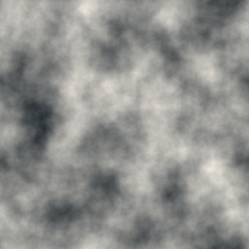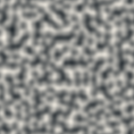Both of these were generated from the same seed. The left has octaves starting with a period of $128$ decreasing exponentially by $\frac{1}{2}$ until 2 (i.e., $7$ octaves) and similarly decaying weights. The right is just one instance of the function with a period of $32$. If you look closely you can see some faint dark spots in the LHS corresponding to the single instance seen on the RHS.

The left figure uses a discrete gradient for colors and 3 octaves starting from 32px per cell. The right uses a continuous gradient between 3 colors and 6 octaves starting from 128px per cell. These GIFs are all made by computing 3D Perlin and animating the z-coordinate.

Voronoi Noise

Both Voronoi noise and Worley noise are applications of the more general concept underlying Voronoi diagrams. They are all primarily concerned with associating all points in a space with their closest site(s). Where sites are just a predefined set of points.

Background

If you match each point in space with its closest site, then you partition the plane into $n$ convex regions, where $n$ is the number of sites.

Formally, a partition in a Voronoi diagram associated with site $i$ in a space $S$ can be defined as follows:

for sites $P_i, i \in \{ 1, ..., n \}$, point $P$, and some distance function $d$. This definition was adapted from the one given at p.1 in A Faster Divide-and-Conquer Algorithm for Constructing Delaunay Triangulations.

In words, a point $P$ is in the partition associated with point $P_i$ if the distance between $P$ and $P_i$ is less than or equal to the distance between it and all other points.

I don't know about you, but whenever I see an interesting effect in computer graphics I tend to think that the process for generating it is complicated. But here you have a very popular visual effect generated by one of simplest concepts possible—it's just grouping points by their closest site.

For the record, I would say more often than not most graphical effects have a fairly intuitive geometric explanation underlying them that makes naive implementations fairly easy. It's the optimization and generalization that often makes them more intimidating.

Voronoi diagrams, for example, have quite a bit of research surrounding them! One simple answer as to why is that deciding which point is closest to some arbitrary point is a fairly common problem in computing that doesn't have a straightforward and efficient solution.²

Algorithm

The following is likely the simplest algorithm for computing a Voronoi over a set of sample points; it really is just finding the minimum distance between sample and site for each sample.

Initialization

1. Pick a finite set of sites, $P \in 2^S$.
2. Assign each site a unique value. Let $v(P_i) = v_i$ represent the function mapping each site to a value.
3. Choose a distance function $d(p_1, p_2)$ to calculate distances between samples and sites. Often Euclidian distance: $d(p_1, p_2) = \sqrt{(p_2 - p_1) \cdot (p_2 - p_1)}$.

Sampling

4. Choose some sample point, $p \in S$.
5. For each site, $s$:
   1. Calculate $d(p, s)$ and compare it to the minimum distance already observed.
   2. If $d(p,s)$ is the smallest distance, record it as well as the site $s_{\text{min}} = s$.
6. Return $v(s_{\text{min}})$.

Relaxing Points

If few sites are being used and they are generated using a uniform distribution, quite often you will find that sites by chance look clumped up or have large voids in areas of your sample space. This results in noticeably larger/smaller Voronoi cells.

To "fix" this, you can relax the points after they are generated and/or increase the site generation area to outside of the viewing area. A common approach for relaxation is to use Lloyd's algorithm, which finds the centroid of each cell/partition, and sets the site of that partition to its centroid. This can be iterated a number of times until sufficient relaxation is achieved.

An exact computation of the centroids is possible, but doing so can be quite complicated. A simpler approach is to start by discretizing the function into the desired sample space by calculating the full Voronoi texture and labeling each sample with its associated site. Then iterate over these points adjusting the centroid of each point's site based on that sample's location.

Examples

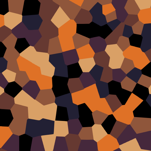Both figures are examples of colored Voronoi diagrams. The left uses the typical Euclidian distance, and the right uses the Manhattan distance ($d(p_1, p_2) = | p_2 - p_1 |$).

Worley Noise

Worley noise is a generalization of Voronoi diagrams. Instead of associating each point in space with the single point that it is closest to, you associate it with its $M$ closest points, and give it a value of some combination of those distances.

In it's simplest form (one site per point, $W(p) = d(p, P)$), Worley can be thought of as simply a continuous representation of a Voronoi diagram.

There is no exact definition of Worley noise in the sense that the term refers more to the family of functions composed of one or more of these distances. For example, the original paper gave the following function as an example:

Where $W_1$ and $W_2$ are basis functions representing the $1^{\text{st}}$ and $2^{\text{nd}}$ shortest distances from $p$, respectively.

Algorithm

The original Worley algorithm generates the points differently than how we handled it in the Voronoi algorithm above. It actually uses a lattice structure (like Perlin noise), where each cell has a number of points generated according to a Poisson distribution uniformly distributed throughout.

The original Worley enforces a minimum of 1 point per cell to ensure that the minimum distance must be within the current cell or adjacent eight (26 in 3D).

This lattice approach also helps to make points more evenly distributed, as opposed to just uniformly generating $n$ points over your entire area, so long as your sample area spans multiple cells.

For a Worley function that uses the $M$ closest distances:

1. Pick a point anywhere in real space, $p$.
2. Calculate the cell that it is in and all adjacent cells.
3. For each cell:
   1. Randomly sample from a $\text{Poission}(\lambda)$ distribution to decide the number of points in the cell, $n_p$.
   2. For each point uniformly generate an offset from the cell corner (generally an offset in $[0,1]$), and calculate its absolute position.
   3. Now for all cell points, calculate their distance from $p$, storing the closest $M$ points observed between all cells.
4. Given the $M$ distances calculate a custom combination of the distances, $W_M(p)$.

Note: as is typical in lattice structures, each cell can have its own unique hash so that whatever random value(s) are associated with it can be recalculated the same each time the cell is encountered.

As an optimization, the original Worley eliminated entire rows of the lattice by inserting some logic based on already observed minimum distances. For example, if our $M^{\text{th}}$ closest distance is some distance less than the distance from our sample point $p$ to the plane below, above, or beside the center cube than we can throw out each of these groups.

Visualizing

Unlike Perlin, the ranges of Worley basis functions are generally not in a fixed range, so there is no trivial way to pick a color from the output. Generally, you will want to scale the values to fit into an easy to work with range like $[0,1]$ and then just pick from a gradient parameterized by the normalized value.

You can achieve this scaling by finding the max value and just dividing all Worley output values by it, but depending on the distribution of your points (e.g., if there is an unusually large distance for one of them) this can wash out your colors. In general, when computing Worley noise an option to clamp values and then scale by the clamp can address this, but what clamp to use is highly situational.

Examples

The animation on the left is just the first basis function for Worley clamped at a distance of $26$. The right is that same basis function (and seed) with gradient flipped. Interestingly, the visual appearance of Worley changes drastically if you simply switch the primary and secondary colors of the gradient used. Here you can see the cells look spherical because the dark edges create an effect of depth.

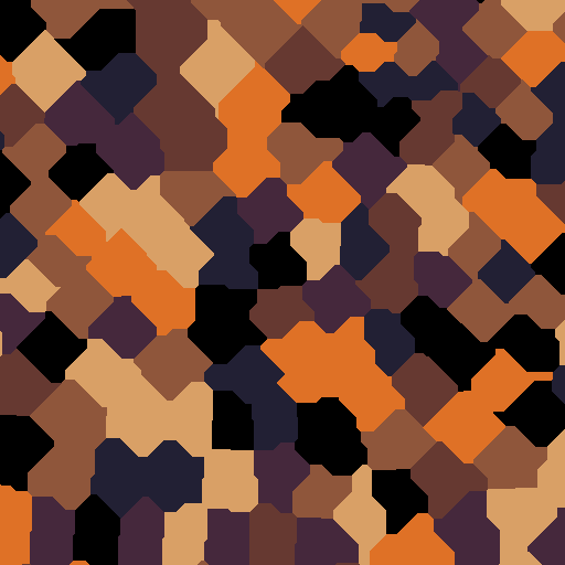
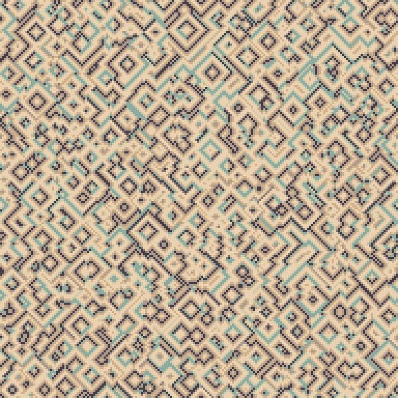
The two figures above use a discrete palette. Left uses the typical Euclidian distance; right uses Manhattan distance and a larger cell size.

The figure on the left uses the first basis Manhattan distance plugged into a $\sin$—the unusual color distribution comes from offsetting the pallet after generation. The right figure uses a simple combination of the first and second basis function: $W_M(p) = d_2(p) - d_1(p)$.

Footnotes

1. Original Perlin uses a finite set of precalculated gradient values, and selects one for a cell by hashing the $\vec c$ coordinate. A simpler, less efficient way is to simply use that hash to generate the points every time you need them (i.e., as a seed). The latter approach also generates "unique" gradients for all cells in the lattice. ↩

2. Delauney triangulation is a common technique for efficiently generating Voronoi diagrams. Delauney triangulation has a few properties that relate it to Voronoi diagrams (or rather each triangulation with a diagram) that makes this technique possible. ↩